i'm annoyed by side channel stuff being fairly inaccessible even though the basic concept isn't that hard to understand so here's a blog post about it (and there will be more later hopefully!!)
side channel?
when you have some crypto algorithms often times you are interested in bonking them, for example by recovering the secret key or making the algorithm accept data that has been tampered with (in traditional parlance, you want to violate properties of Confidentiality, Integrity, and Authenticity). crypto code can have software bugs: if you think about code as a specification of what a program is supposed to do, there can be cases where the specification is simply wrong. but even if the specification is perfectly correct, and would execute flawlessly on an ideal computer, there can still be vulnerabilities in running the code on an actual computer that can still violate important security properties
here's some code
const char* password = getenv("THE_PASSWORD");

bool check_password(char* input) {
    if (strlen(input) != strlen(password)) return false;
    for (size_t i = 0; i < strlen(password); i++) {
        if (input[i] != password[i]) return false;
    }
    return true;
}
suppose you want to figure out what the password is.... how can you do that? there's nothing wrong with the specification of the algorithm (comparing a password to a correct password -- i mean what could possibly go wrong)
but there's a problem with the implementation
as soon as you get a character wrong it immediately bails and returns false. so a password that has more correct characters takes more time to check than a password that has fewer correct characters. thus you can mount an attack where you guess the first character, and go with the guess that takes the longest to check, then guess the second character, and select the one that takes the longest to check, and so on until you have guessed all the characters
this is what people like to call a timing side channel, and it turns out that you can even do things with timing like guess AES keys by correlating the time it takes to do AES encryptions of random messages to the expected time it would take for cache lookups in the CPU while it's processing the encryption (however, modern CPUs contain hardware AES logic that largely solves the cache timing issue)
anatomy of a side channel attack
ingredients1
- a secret you need to know
- input to the code that you control
- some sort of measure of the code being executed besides just the input and output
the key part is that when the secret combines with your input, this affects some side channel measurement in a way that you can observe. and if you can figure out how that measurement changes with different combinations of your input and the secret, then you have a model for guessing what the secret is. in the timing example, we could develop a model where we said the following
if more characters in our guess prefix match the real secret, then the algorithm will take longer to execute
we reverse that, and now we know that if we measure a longer execution time, that means our input must have been closer to being correct
hardware side channel leakage
ok so timing is cool and all but one interesting aspect of actual cryptography on actual hardware, like a microcontroller, is that the microcontroller uses electricity to perform its computations (shocking, i know). more interestingly, the amount of current it draws can be dependent on what exactly it's calculating. correspondingly, it can emit unintentional radio waves as a result of what it's running on the chip as well
these are both some great side channels to use in order to examine what's going on inside a chip when you don't have the capability to decap and microprobe the actual silicon. basically, you can measure power consumption or electromagnetic emissions on a chip, and those signals will contain some information that can be used to recover what the data the chip is processing actually is (like, crypto keys for AES, cause y'know that sounds juicy)
there are two root causes for leakage that are widely used as models that can tell you what the leakage measurement should look like given a certain data value
- hamming weight. this counts the number of
1bits in the binary representation of a number. this is because, in silicon, 1 bits are represented by a high signal and 0 bits are represented by a low signal, which means that if a data bus inside the chip is transmitting the data you're interested in, then it's going to use an amount of power for that bus that is proportional to the number of "on" wires in the bus, which is the number of1bits in the value - hamming distance. this counts the number of changed bits between two numbers. this happens because changing the value of a register in the CPU (which can happen when code sets a variable to a different value) will use an amount of power proportional to the number of bits that changed during that update. in order to use hamming distance as a model you need to inspect the assembly-level code that is executing on the CPU to know when specific registers change values that you can model this way (or you can guess -- in general it's going to be more complex than hamming weight but can return better results for certain chips)
AES encryption
suppose we have an implementation of AES on a microcontroller and we want to know the secret key used for the AES, and we have some setup that allows us to capture hardware side channel data. this is going to consist of a high speed measurement of the chip's power consumption, or a measurement of an EM probe placed over the chip (ideally near an area of the silicon where you might know your data is being processed -- EM data is also going to need additional filtering and demodulation depending on the exact target hardware and setup). the main component of capturing hardware side channel signals is just a high speed analog-digital-converter of some kind that can record the analog characteristics of the target device (current drawn by the chip, or EM emissions from the chip) very fast. so for capturing this data, people like to use oscilloscopes that can connect to your computer, like a PicoScope. alternatively, the ChipWhisperer is an oscilloscope-like device for side channel education/training
then we have the basic ingredients
- secret you want to know: the key lol
- input: some plaintext which you can feed to the encryption
- measurement of the algorithm: hardware side channel data
- model to predict the measurement values for different inputs: hamming weight or distance (for this post i am going to focus on hamming weight)
more specifically, the AES encryption algorithm has a step in the first round where it combines the key with the input by XOR of the key and the plaintext (AddRoundKey) and then a step where these values are passed through a substitution box (SubBytes). so basically, you can think of AES like this
void AES_encrypt(byte key[16], byte plaintext[16]) {
    byte output[16];
    // ... some stuff ...
    // AddRoundKey
    for (size_t i = 0; i < 16; i++) output[i] = key[i] ^ plaintext[i];
    // SubBytes
    for (size_t i = 0; i < 16; i++) output[i] = sbox(output[i]);
    // more steps, and more rounds....
    // etc
}
so to develop the model, first we figure out what the value we are targeting is, this should be a value that combines the input and secret (and it's helpful to have a non-linear operation you are targeting, because this reduces the possibility of false positives in your results. the AES sbox is very non-linear). we're going to be attacking each byte of the key individually, so in the following i will assume you have picked a byte to bonk. you can obviously repeat this same attack with the same data for each key byte. here's the model:
for a certain secret key byte and input byte, the code will at some point compute the value
sbox(keybyte ^ inputbyte)
now, we just wrap that in the hardware leakage model (let's say hamming weight): hamming(sbox(keybyte ^ inputbyte))
and yeah that's it, now we have the ability to predict what the leakage should look like given the inputs to the encryption
setting up
i assume people generally don't just have a ChipWhisperer on hand to collect some real traces. luckily some good people have prepared a database of AES side channel traces collected on an AVR smartcard platform (it's meant for training machine learning models, but it's also a useful demo dataset)
you can get the data here: https://github.com/ANSSI-FR/ASCAD/tree/master/ATMEGA_AES_v1/ATM_AES_v1_fixed_key
one thing to note is that this is using AES which is masked. masking is a protection against side channel attacks by introducing randomness which is unknown to the attacker on each run of the algorithm, which messes with our ability to predict leakage measurements. so to start, we're going to cheat and use the mask values recorded in the database as if they were known by the attacker, but i will later demonstrate how to bonk the key without knowing the masks
we're going to use python, and you'll need the standard numpy, scipy, matplotlib, and to read the data format, h5py
performance
this can go very fast if you install OpenBLAS. on manjaro, this is the openblas package (NOT blas -- that's the reference implementation and it is quite literally 20 times slower)
on debian and friends i believe the package is sudo apt-get install libopenblas-dev
alignment
the traces in the ASCAD.h5 database are aligned, which means that every trace (consisting of a series of integers 0-255 reflecting the analog measurements by time) represents starting at exactly the same point relative to the AES operation being performed in the code. when capturing traces, even with very precise triggering to start recording right when the operation you're attacking starts, it can be hard to end up with perfectly aligned traces because of environmental variables outside of your control. so typically some alignment of what you captured is necessary, to make sure every trace's time axis lines up exactly with the rest. for the correlation-based attack here, it's important to make sure the traces are aligned. even 10% of your traces being badly aligned can completely throw off the attack
ASCAD also provides some "desynced" databases, which have been artificially misaligned, which i'll use here to demonstrate trace alignment as in a real attack. to align traces, we can use (FFT) signal convolution (scipy.signal.correlate) to compute the best alignment for the traces fairly quickly. one issue when doing this with ASCAD which i noticed is that because the traces are very periodic, the best correlation according to scipy.signal.correlate can be shifted one period sometimes. however, if we take N best correlations and test the Pearson correlation coefficient of each one, then picking the alignment with the highest Pearson correlation seems to get good results
when doing this on real data, it can also be helpful to use the Pearson correlation to throw away garbage traces (ones where the best Pearson correlation is too low, according to some cutoff). you're going to have some of those and you don't want them to be in the data
open the database (we'll use the attack traces section. for our purposes there is no difference between the profiling and attack parts). also, we're only dealing with the first 1000 traces
db = h5py.File("./ASCAD_databases/ASCAD_desync100.h5", "r")["Attack_traces"]
ntraces = 2000
alignments = numpy.zeros(ntraces, "int64")
pick the first trace as a reference trace (make sure to convert it to double. the database stores traces as u8, which will cause all calculations to wrap and be screwed up)
reference = traces[0].astype("double")
scipy provides correlation_lags which computes a vector of offsets corresponding to the output of correlate which can be used to determine which alignment offset ("lag") corresponds with a correlation value. we can use this to shift our traces forwards or backwards to match the best alignment
lags = scipy.signal.correlation_lags(len(reference), len(reference))
now do the alignment on every trace skipping the first one (that has an alignment of 0, since it is the reference). here there is some code that uses a second pass to maximize the Pearson correlation for the top 10 FFT correlation peaks
    for i in tqdm.trange(1, ntraces):
        trace = traces[i].astype("double")
        corr = scipy.signal.correlate(reference, trace)

        max_idxs = corr.argsort()[-10:][::-1]
        max_corr = 0
        max_idx = -1
        for idx in max_idxs:
            lag = lags[idx]
            if lag == 0:
                s_ref = reference
                s_trs = trace
            elif lag < 0:
                s_ref = reference[:lag]
                s_trs = trace[-lag:]
            else:
                s_ref = reference[lag:]
                s_trs = trace[:-lag]
            pcorr = numpy.corrcoef(s_ref, s_trs)[1,0]
            if pcorr > max_corr:
                max_corr = pcorr
                max_idx = idx

        lag = lags[max_idx]
        alignments[i] = lag

    alignments -= numpy.min(alignments)
we can use the alignments to produce a matrix of aligned traces
    traces = numpy.zeros((ntraces, 800), 'double')
    for i in range(ntraces):
        traces[i, alignments[i]:alignments[i]+700] = db["traces"][i]
visualizing is always helpful, so let's plot 10 traces
    for i in range(10):
        plt.plot(traces[i], color=numpy.hstack((numpy.random.random(3), [0.5])))
    plt.show()
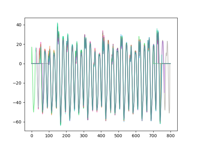
you can see here in the central part of the plot every trace lines up very well. most of the traces are layered on top of each other, and each of the peaks are roughly the same shapes. this indicates that we have a consistent time axis with respect to the AES encryption operation happening on each trace
if your dataset contains some garbage (ASCAD, helpfully, doesn't) then there is a chance you will pick a garbage reference trace. you'll notice then that all your correlations will be very low, and in that case you can try picking a different reference trace
guessing
now we have aligned traces. somewhere in the trace, at some time point, there is a leakage for our model (recall that the model was hamming(sbox(keybyte ^ inputbyte)). now since ASCAD has masks we're going to cheat and add in the mask value (for an actual attack, this would be unknown -- stick around), making the model hamming(sbox(keybyte ^ inputbyte) ^ mask). (in ASCAD, the mask byte for the sbox output is the last byte of the masks array for an entry in the database)
now... we have the inputbyte available for each trace. but what about keybyte? well it's a byte, so it could be from 0 to 255. that's low enough for us to just guess every possible key byte
so we end up with 256 guesses, where guess i is hamming(sbox(i ^ inputbyte) ^ mask)
let's make that model (because i like yak shaving, i implemented an interface to __builtin_popcount() in numpy which you can find here. do a pip3 install --user -e .). here, we're using the 3rd key byte (2, starting at 0) because it's the first masked key byte -- the first two are unmasked and were used for validation -- and we're going to attack the same one later without knowing masks. also, we use the last mask byte which was used in the AES implementation to mask the s-box output
    model = numpy.repeat(numpy.arange(256, dtype='uint8'), ntraces).reshape((256, ntraces))
    for i in tqdm.trange(ntraces):
        (pt, ct, key, mask, desync) = db["metadata"][i]
        pt_v = pt[2]
        mask_v = mask[15] # cheating here
        model[:, i] = AES_SBOX[model[:, i] ^ pt_v] ^ mask_v
    model = numpy_popcount.popcount(model).astype("double").transpose()
the model contains a value for each key guess, and for each trace we're analyzing. thus one of the key guesses will very nicely predict the values at a specific tick of the trace set. it's also important to make sure you convert to double because if you leave the data type as int then you will have problems in the next steps
so the job is to find which key byte and which tick index are actually matching. one way to do that is to compute the Pearson correlation coefficient between every key guess of your model, and every tick guess of the data. then, get the maximum correlation coefficient, and it should give you the correct key byte and tick index where the leakage occurred2
there's a slow way to do this, just use numpy.corrcoef using a vstack of the model and traces sets, and then select a corner of the output matrix which will be the correlation values you're looking for. this is unfortunately more RAM-intensive than we really want -- it outputs a full (ntraces + 256)**2 size square matrix when we really need the 256 by ntraces corner. because of this i decided to go see how pysca 3 did things and (pysca is fairly unintelligible honestly) found this implementation which i adapted into the following more optimized code, which goes very fast with openblas4
class Correlator:
    def __init__(self, P):
        self.P = P - numpy.mean(P, axis=0)
        self.tmp1 = numpy.einsum("nm,nm->m", self.P, self.P, optimize='optimal')
        self.P = self.P.transpose()

    def corr_submatrix(self, O):
        O -= numpy.mean(O, axis=0)
        numerator = self.P @ O
        tmp2 = numpy.einsum("nt,nt->t", O, O, optimize='optimal')
        denominator = numpy.sqrt(numpy.outer(self.tmp1, tmp2))
        return numerator / denominator
this is a class because it remembers the parts of the computation for the model matrix, which allows the corr_submatrix method to be called multiple times with chunks of data (chunked along the tick axis), and the results concatenated. chunking is useful to avoid eating up tons of RAM, at the cost of performance
now just call it
    # uwu
    correlator = Correlator(model)
    coefs = correlator.corr_submatrix(traces)
    coefs = numpy.abs(coefs)
we use the absolute value because when looking for peaks, correlations could be negative (they would not be in this case, but for other types of leakages you might want to catch highly negative correlations as well)
the output is a 256-by-nticks matrix, and the correlation at i,j represents key guess i with tick j
collect the max correlations along the key guess axis and plot it
    max_by_key = numpy.max(coefs, axis=1)
    plt.plot(max_by_key)
    plt.show()
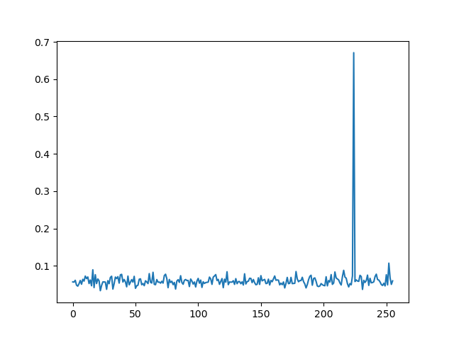
yeah. the secret byte is very obvious here, and indeed if you check the x-axis for the peak you'll see it's 0xe0, which is matches the real 3rd key byte
and in practice you'd just repeat this for all 16 key bytes
that was easy -- but wait we cheated!
ok so now we do it without knowing the mask (a more realistic attack scenario). the problem is, the mask is randomized, so if our model says hamming(sbox(keybyte ^ inputbyte)), it's not going to match very well with reality, and we're not going to see any peak in the max correlation plot. in fact you can see this if we remove the cheating from the previous code
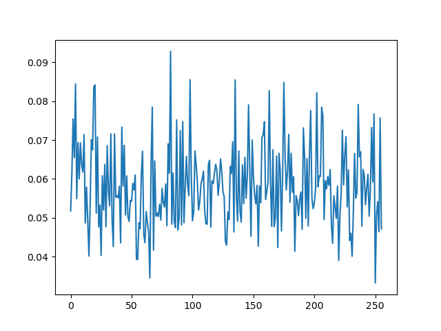
you can see there is no obvious peak here -- the attack failed
the way to bypass masking is to do what is called a second-order attack. "order" here just means how many points along the time axis you consider at a time. so you might have noticed in the previous section we calculated correlation by a key guess axis and a tick axis, and the result of that was a high correlation value at one specific key guess and one specific tick. in a second-order attack, however, we make combinations of 2 ticks (and an N-order attack would use combinations of N ticks)
to make the combinations of two ticks, we take the absolute difference between the values at both ticks for each trace. this results in a new trace of n*(n-1)/2 values, where each value is the absolute difference between 2 unique values of the original trace
the reason this works is because inevitably with masking, there is going to be some second tick in the traces that is correlated with the mask value. we don't know what the mask value is, but we can use that second tick to subtract the leakage of that mask value from the leakage of the s-box operation (since the state is xor'd with the mask, this corresponds somewhat with a sum of hamming weights, over a large number of random mask values), which would then correlate very well with the unmasked key guesses in the model
first, we'll make a model without cheating
    model = numpy.repeat(numpy.arange(256, dtype='uint8'), ntraces).reshape((256, ntraces))
    for i in tqdm.trange(ntraces):
        (pt, ct, key, mask, desync) = db["metadata"][i]
        pt_v = pt[2]
        model[:, i] = AES_SBOX[model[:, i] ^ pt_v]
    model = numpy_popcount.popcount(model).astype("double").transpose()
and now, make second-order combinations of two ticks as described
    nticks = traces.shape[1]
    traces_x = numpy.zeros((ntraces, nticks*(nticks - 1)//2), 'double')
    tx_i = 0
    for i in tqdm.trange(nticks):
        for j in range(i+1, nticks):
            traces_x[:, tx_i] = numpy.abs(traces[:, i] - traces[:, j])
            tx_i += 1
you can see here the absolute difference is being used to generate this new second-order dataset, where the "tick" axis is now a "combination of 2 ticks" axis
now that we have the second order combinations it's the same thing (this time, we split up the data into sequential chunks to lower the RAM usage)
    correlator = Correlator(model)
    ncolumns = 4
    step = traces_x.shape[1] // ncolumns
    all_coefs = []
    for i in tqdm.trange(ncolumns):
        start = i * step
        end = (i + 1) * step
        coefs = correlator.corr_submatrix(traces_x[:, start:end])

        all_coefs.append(coefs)

    all_coefs = numpy.hstack(all_coefs)
    all_coefs = numpy.abs(all_coefs)
on my computer (skylake laptop, with openblas) this runs in seconds
and now do the same plot along the key axis
    max_by_key = numpy.max(all_coefs, axis=1)
    plt.plot(max_by_key)
    plt.show()
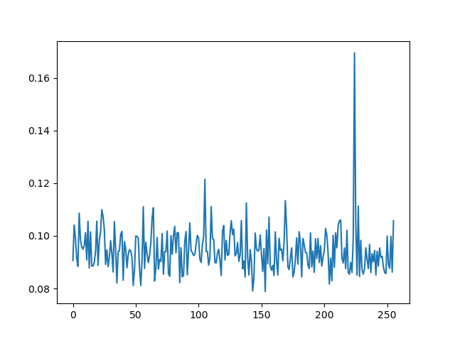
you can see the peak is not as high as before, but it's still very much distinguishable5
one important thing about this is, the more traces you have, the lower the noise floor is going to be. having a low number of traces can result in a plot which doesn't have a clear correct guess on it, even if the leakage is present and correctly analyzed. this becomes important especially when you are analyzing leakage that is not as obviously non-linear as the AES s-box. you can see if you run this second order attack with 1000 traces instead of 2000, the peak will be much less obvious (and barely the maximum). and if you run it with 3000, the peak will become more obvious
the other thing to realize is that the correlation can reveal correct secret values if you have literally any advantage in your model over the noise floor. if you can guess leakage in your model better than pure randomness even just sometimes, then with enough traces you'll be able to leak the secret. the correlation attack is extremely powerful and very fast. even for a (quadratically scaling) second-order combination of ticks in your trace data
ok great, gimme the code
the full code is available at https://git.lain.faith/haskal/gist/src/branch/gist/sca/ascad
:wq
now, go hack yourself some AES keys for great good
or other stuff. i wanted to develop a from-scratch HMAC-SHA256 attack and maybe XChaCha20 too but i haven't gotten to it yet (these are more involved because they require more leakage steps of more linear operations -- like addition and xor, which are hard to deal with)
acknowledgements
i would like to extend a big thanks to Taowa for providing helpful feedback on this post
we're going to focus on non-profiled side channel attacks, which means you just get a trace set with varying inputs and you have to find the secret. there's also a class of profiled side channel attacks, which have the capability for the attacker to use a copy of the system to perform analysis on traces where the secret and input are both known, and then use that information to attack the attack system where the secret is unknown. most importantly, attacks based on deep learning (that's where the ASCAD database we will use comes from)
there are other ways to do this, like traditional differential power analysis, which bins the traces based on bits, or mutual information analysis, which just uses another statistical measure (mutual information, as you might guess). but here we're going to use the correlation method
an influence/precursor of the better known jlsca
pysca is available under a GPL-3.0 license which you can find in the repo. my implementation is also licensed under GPL-3.0
the reason it's not as high is because the assumption we made that XOR operations correspond with a sum of hamming weights and thus subtracting hamming weights is sufficient to unmask a leakage value is not exactly correct. but over a large number of random inputs it will be good enough that there is still some correlation we can observe

Comments
No comments yet. Be the first to react!