continuing to make some sort of sense out of side channel literature that is out there, here's another cool trick with actual code
one of the issues with doing time-domain side channel analysis is that all your traces need to be perfectly aligned. this can prove challenging, especially if the target has side channel countermeasures that include random delays in the sensitive code to throw off alignment. what can you do about that? well you could do your analysis in the frequency domain instead of the time domain
frequency domain?
typically side channel traces are a relation between time and the power consumption (or RF emanations) at that time. using a Fourier transform1, this can be converted into a relation between various frequencies and their amplitude and phase (which when added together form the original signal2). the side channel leakage, at least for first order attacks, can still show itself in the frequency-domain version of the data, and thus can be extracted that way. the important thing is in the frequency domain we don't actually care about trace offset at all. trace alignment is irrelevant because in the frequency domain, the only difference between two signals that are identical but offset by some amount of time is the phase of the resulting frequency bins (and we ignore phase)
ok let's do it
first some probably familiar code if you've seen the previous post. we're using the ASCAD_desync100 dataset and taking 2000 traces out of that (also using the mask metadata)3
ntraces = 2000
db = h5py.File("./ASCAD_databases/ASCAD_desync100.h5", "r")["Attack_traces"]
traces = db["traces"][0:ntraces, :].astype("double")

logger.info("making first order model")
model = numpy.repeat(numpy.arange(256, dtype='uint8'), ntraces).reshape((256, ntraces))
for i in tqdm.trange(ntraces):
    (pt, ct, key, mask, desync) = db["metadata"][i]
    pt_v = pt[2]
    mask_v = mask[15]
    model[:, i] = AES_SBOX[model[:, i] ^ pt_v] ^ mask_v
model = numpy_popcount.popcount(model).astype("double").transpose()
ok now the fun part, transform all the traces with scipy.fft, take the absolute value of the result to discard phase information, and then take the top 50 peaks which we assume contain the leakage4
fft_traces = numpy.zeros(traces.shape, traces.dtype)
for i in range(traces.shape[0]):
    fft_traces[i, :] = numpy.abs(scipy.fft.fft(traces[i, :]))

traces = fft_traces[:, 1:350]
avg = numpy.mean(traces, axis=0)
peaks = avg.argsort()[-50:][::-1]
traces = numpy.hstack([traces[:, i:i+1] for i in peaks])
with this, do the typical correlation analysis as before, just like if traces represented the original time-domain trace set
correlator = Correlator(model)
coefs = correlator.corr_submatrix(traces)
coefs = numpy.abs(coefs)
max_by_key = numpy.max(coefs, axis=1)
plt.plot(max_by_key)
plt.show()
results
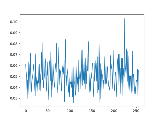
this is a lot more noisy than the time-domain attacks where we took care to align the traces, but the point is we still get the right key byte without any trace alignment being actually necessary, which makes this a really powerful kind of attack
the code (+ previous code) can be found here https://git.lain.faith/haskal/gist/src/branch/gist/sca/ascad/attack.py
approximately. computers aren't able to calculate perfect Fourier transforms (mitigating this requires windowing, which tries to remove the artifacts from the result and there are various kinds of windows you can use with Fourier transforms, but for now ignoring windows is fine)
you might also notice the [1:350] slice. this is because in this analysis, we discard the 0Hz frequency bin ("DC") because it's not interesting, and the result of running FFT is symmetric so we don't actually need the top half as it mirrors the bottom half
this is similar to the previous post's first order attack. second-order frequency domain attacks require different leakage modelling and it's more complicated. also i haven't written the demo for that yet
an intuitive way to see what a Fourier transform is actually doing is to think about a music visualizer. classic music visualizers have bars corresponding to different frequencies, and the height of each bar indicates how loud that frequency is within the music. visualizers like that are doing Fourier transforms internally to produce that visualization. the important thing is you can do that with any sort of data, not just audio

Comments
No comments yet. Be the first to react!